Friday, December 20, 2013

HCUP and Python Pt 5: Nulls and Pre-Analysis

This is the fifth post in a series on working with Healthcare Cost and Utilization Project (HCUP) datasets using Python and other open-source alternatives to SAS and SPSS, which are the two primary data tools supported by HCUP.

Please note! These instructions build off previous posts. In particular, they assume you are configured with Canopy and PyHCUP, have some basic facility with Python/IPython, and have already read in a small HCUP dataset.

IPython Notebook from this Tutorial

You can download an IPython notebook with code examples from this post.

Now that you have some HCUP data read in, you'll want to do a little housekeeping to get it ready for meaningful analysis. This post will cover two data wrangling tasks you're probably all-too-familiar with: identifying missing values and characterizing/verifying the contents of the data set.

HCUP Sentinel Values

Files from HCUP have several different sentinel values used to mark missing, invalid, or otherwise unavailable data. For a full breakdown, see HCUP's documentation on missing values in http://www.hcup-us.ahrq.gov/db/coding.pdf. In most of my work, the details of this are not vital I just need to mark them as null in the data set.

Replacing Sentinel Values

PyHCUP has a built-in function in its parser module to sweep through an imported HCUP data set and mark all the sentinels as missing values. To use it, pass your imported data set to the parser.replace_df_sentinels() function. This may take some time, depending on the size of the data set you've imported and the speed of your computer.

In [4]:nulls_replaced = pyhcup.parser.replace_df_sentinels(df)

Check the AGE column (or whichever column you used .describe() with previously) in the replaced and non-replaced data to see the effects.

In [5]:df['AGE'].describe() #before Out[5]:count 10000.000000 mean 43.053200 std 25.857201 min -88.000000 25% 24.000000 50% 46.000000 75% 63.000000 max 104.000000 dtype: float64 In [6]:nulls_replaced['AGE'].describe() #and after Out[6]:count 9999.000000 mean 43.066307 std 25.825253 min 0.000000 25% 24.000000 50% 46.000000 75% 63.000000 max 104.000000 dtype: float64

Notice that, in my data set, the count for this column has dropped by one. When using .describe() on a column, the count reflects the number of non-null values. When I used parser.df_replace_sentinels(), it found and replaced only one sentinel value in the AGE column. Note as well that the minimum value in this column has changed from -88 to 0, which is still young but no longer requires time travel.

Characterizing Numeric Data

Although we are only looked at one column above for brevity, the parser.df_replace_sentinels() function has been applied to every column in the data set. You check describe additional columns by substituting in the column name for AGE in the code we've been using so far. Here is another, looking at the total charges per inpatient stay.

In [7]:nulls_replaced['TOTCHG'].describe() Out[7]:count 10000.00000 mean 32321.22250 std 50510.43668 min 990.00000 25% 9669.00000 50% 18253.50000 75% 35106.25000 max 1162225.00000 dtype: float64

So out of these 10,000 stays, somebody got out for cheap at less than $1,000 and somebody had a rough time with a bill greater than $1.1 million.

It is possible to describe multiple columns side by side by first preparing a list of columns, then referring to that instead of passing a single column name. In Python, you can make a list by putting all the desired list items in a shared set of square brackets, with commas between the items. For example, we could get ages, total charges, and length of stay all at once with something like this.

In [8]:col_list = ['AGE', 'TOTCHG', 'LOS'] In [9]:nulls_replaced[col_list].describe() Out[9]:
 AGETOTCHGLOS
count9999.00000010000.0000010000.000000
mean43.06630732321.222506.110600
std25.82525350510.4366810.319303
min0.000000990.000000.000000
25%24.0000009669.000002.000000
50%46.00000018253.500003.000000
75%63.00000035106.250006.000000
max104.0000001162225.00000271.000000

Characterizing Non-Numeric Data

Averages, extreme values, and percentiles are less helpful for describing things like discharge destinations and diagnoses. For non-numeric data, pandas has a built-in .value_counts() method you can use on columns similar to .describe(). As an example, HCUP SID data typically have available a FEMALE column, where a value of 1 indicates the patient was female and 0 indicates the patient was male.

In [10]:nulls_replaced['FEMALE'].value_counts() Out[10]:1 5142 0 4857 dtype: int64

Unlike .describe(), you cannot directly use .value_counts() simultaneously with multiple columns. However, you can use Python to put together a loop that generates value counts for columns in a list. You can also "nest" this kind of count by grouping, such as getting value counts of primary diagnosis by race or discharge destination by homeless status. We'll cover both of these techniques in future posts.

Knowing What Columns Are Available

HCUP provide documentation with detailed descriptions on which columns are available for which states in which year, as well as what the contents of each column mean. But for day-to-day work, we can get a list of all the columns in a DataFrame by invoking DataFrame.columns on any of our data sets. The results should be the same right now whether you use it on df or nulls_replaced, since one is derived from the other.
In [11]:nulls_replaced.columns Out[11]:Index([AGE, AGEDAY, AGEMONTH, AHOUR, AMONTH, ANESTH, ASOURCE, ASOURCEUB92, ASOURCE_X, ATYPE, AWEEKEND, BLOOD, BWT, DHOUR, DIED, DISPUB04, DISPUNIFORM, DISP_X, DQTR, DRG, DRG24, DRGVER, DRG_NoPOA, DSHOSPID, DX1, DX2, DX3, DX4, DX5, DX6, DX7, DX8, DX9, DX10, DX11, DX12, DX13, DX14, DX15, DXCCS1, DXCCS2, DXCCS3, DXCCS4, DXCCS5, DXCCS6, DXCCS7, DXCCS8, DXCCS9, DXCCS10, DXCCS11, DXCCS12, DXCCS13, DXCCS14, DXCCS15, DXPOA1, DXPOA2, DXPOA3, DXPOA4, DXPOA5, DXPOA6, DXPOA7, DXPOA8, DXPOA9, DXPOA10, DXPOA11, DXPOA12, DXPOA13, DXPOA14, DXPOA15, ECODE1, ECODE2, ECODE3, ECODE4, ECODE5, ECODE6, ECODE7, ECODE8, ECODE9, E_CCS1, E_CCS2, E_CCS3, E_CCS4, E_CCS5, E_CCS6, E_CCS7, E_CCS8, E_CCS9, E_POA1, E_POA2, E_POA3, E_POA4, E_POA5, E_POA6, E_POA7, E_POA8, E_POA9, FEMALE, HCUP_ED, HCUP_OS, HISPANIC_X, HOSPBRTH, HOSPST, Homeless, KEY, LOS, LOS_X, MDC, MDC24, MDNUM1_R, MDNUM2_R, MEDINCSTQ, NDX, NECODE, NEOMAT, NPR, PAY1, PAY1_X, PAY2, PAY2_X, PAY3_X, PL_CBSA, PL_MSA1993, PL_NCHS2006, PL_RUCA10_2005, PL_RUCA2005, PL_RUCA4_2005, PL_RUCC2003, PL_UIC2003, PL_UR_CAT4, PR1, PR2, PR3, PR4, PR5, PR6, PR7, PR8, PR9, PR10, PR11, PR12, PR13, PR14, PR15, PRCCS1, PRCCS2, PRCCS3, PRCCS4, PRCCS5, PRCCS6, PRCCS7, PRCCS8, PRCCS9, PRCCS10, PRCCS11, PRCCS12, PRCCS13, PRCCS14, PRCCS15, PRDAY1, PRDAY2, PRDAY3, PRDAY4, PRDAY5, PRDAY6, PRDAY7, PRDAY8, PRDAY9, PRDAY10, PRDAY11, PRDAY12, PRDAY13, PRDAY14, PRDAY15, PROCTYPE, PSTATE, PSTCO, PSTCO2, PointOfOriginUB04, PointOfOrigin_X, RACE, RACE_X, TOTCHG, TOTCHG_X, YEAR, ZIP3, ZIPINC_QRTL, ZIP, AYEAR, DMONTH, BMONTH, BYEAR, PRMONTH1, PRMONTH2, PRMONTH3, PRMONTH4, PRMONTH5, PRMONTH6, PRMONTH7, PRMONTH8, PRMONTH9, PRMONTH10, PRMONTH11, PRMONTH12, PRMONTH13, PRMONTH14, PRMONTH15, PRYEAR1, PRYEAR2, PRYEAR3, PRYEAR4, PRYEAR5, PRYEAR6, PRYEAR7, PRYEAR8, PRYEAR9, PRYEAR10, PRYEAR11, PRYEAR12, PRYEAR13, PRYEAR14, PRYEAR15], dtype=object)

Tuesday, December 10, 2013

HCUP and Python Pt 4: Reading in Data

This is the fourth post in a series on working with Healthcare Cost and Utilization Project (HCUP) datasets using Python and other open-source alternatives to SAS and SPSS, which are the two primary data tools supported by HCUP.

This post will cover how to actually get an HCUP data set into Python. Please note! These instructions assume you have Canopy up and running and have installed the PyHCUP package using pip. If any of those things sound unfamiliar, please visit the second post for instructions on getting set up.

IPython Notebook from this Tutorial

You can download an IPython notebook with code examples from this post.

Locate Your HCUP Data (and decompress it, if necessary)

HCUP Data typically arrive on a DVD, and may or may not be compressed in a ZIP archive. Pick a directory on your computer and copy into it your data file. If the data are in a ZIP archive, extract them at this time. You should end up with a file somewhere around five to fifteen times larger (in MB) than the ZIP archive.

The decompressed file should end in a .asc file extension, though the file extension may be hidden from view depending on your operating system settings. Its name should correspond to the data it contains. For example, you are working with New York's 2008 State Inpatient Database CORE data, you should end up with a file called something like NY_SID_2008_CORE.asc. Make a note of its location as we'll need to know that later.

Locate a SAS Load Program Your HCUP Data

Next, you'll need the appropriate SAS Load Program for your particular HCUP data. Continuing with the above example, we need to find the New York SID 2008 CORE data SAS loading program. HCUP provides SAS loading programs in a few different places on its website, depending on whether you which data you are using. Use the links below to locate the appropriate SAS Load Program for your data. If the links don't work, HCUP has probably changed its website; Google should still be able to help you find them.

After you locate and download the appropriate SAS Load Program for your data, make a note of its location as we'll need to know that later.

Start a New IPython Notebook

Open Canopy and start the Editor. Once the Editor is open, use the "File>>New" menu to start a new IPython notebook. You should save your notebook at this time as well, which may require the use of "File>>Save As".

Write Some Code

Type and run these cells using Shift+Enter after the "In" section of each one. You can omit lines beginning with the pound sign (#), which are comments for clarity. Your output (if any) should look similar to the output in the example.

Import the PyHCUP Package

In [1]:import pyhcup

Specify the Location of Your Files

The formatting for these varies slightly depending on your operating system. Change the path to reflect the correct directory for your files. Also, swap out the filenames at the end for your own!

Paths in Windows look like this.

In [2]:#for Windows, use this style data_path = 'C:\\path\\to\\files\\NY_SID_2008_CORE.asc' load_path = 'C:\\path\\to\\files\\NY_SID_2008_CORE.sas'

Paths in Mac and Linux environments look like this.

In [2]:#for Mac and Linux, use this style data_path = '/home/user/dir/NY_SID_2008_CORE.asc' load_path = '/home/user/dir/NY_SID_2008_CORE.sas'

Acquire Metadata

The SAS Load Program files supplied by HCUP are built to tell SAS how to load your data. We will use them instead to tell Python how to load your data.

In [3]:#build a pandas DataFrame object from meta data meta_df = pyhcup.sas.meta_from_sas(load_path)

You can verify that the meta data we have parsed out is reasonable by calling the meta_df DataFrame object we've created. This summary output is for the 2008 NY SID CORE, referenced above.

In [4]:meta_df Out[4]:<class 'pandas.core.frame.DataFrame'> Int64Index: 222 entries, 0 to 221 Data columns (total 6 columns): field 222 non-null values informat 222 non-null values position 222 non-null values format 6 non-null values label 222 non-null values width 222 non-null values dtypes: int32(1), object(5)

The number of entries reflects the number of columns specified in the SAS Load Program. There should generally be either above more than one hundred or fewer than ten columns, depending on the type of HCUP data. For your own interest, you can see the first x rows in a pandas DataFrame by using its .head() method. If there are too many columns, pandas will abridge this from a table-style output to a summary-style output as seen above.

In [5]:meta_df.head() Out[5]:
 fieldinformatpositionformatlabelwidth
0AGEN3PF.1NoneAge in years at admission3
1AGEDAYN3PF.4NoneAge in days (when age < 1 year)3
2AGEMONTHN3PF.7NoneAge in months (when age < 11 years)3
3AHOURN4PF.10Z4.Admission Hour4
4AMONTHN2PF.14NoneAdmission month2

Use the Metadata to Parse the Data

Now that we have the metadata, we can parse the actual data using the pyhcup.sas.df_from_sas function, with our meta_df as the second our argument. However, given the size of the data sets being read in, you may wish to consider reading in only a subset of rows. Do this by passing an nrows argument as well.

In [6]:#grab the first 10,000 rows in a DataFrame df = pyhcup.sas.df_from_sas(data_path, meta_df, nrows=10000) df Out[6]:<class 'pandas.core.frame.DataFrame'> Int64Index: 10000 entries, 0 to 9999 Columns: 222 entries, AGE to PRYEAR15 dtypes: float64(30), int64(148), object(44)

You now have ten thousand rows from the data file of your choice in a pandas DataFrame object.

The Catch and Next Steps

pandas provides a fantastic set of tools for working with data. One of which is, of course, a simple summary statistics method called .describe() which you can use on either an entire DataFrame or on any of its columns (aka Series). Try it now with the AGE column if you are working with CORE data, or a column of your choice for other data sets. Access any of the columns by using the DataFrame['Column Name (Series)'] notation.

In [7]:df['AGE'].describe() Out[7]:count 10000.000000 mean 43.053200 std 25.857201 min -88.000000 25% 24.000000 50% 46.000000 75% 63.000000 max 104.000000 dtype: float64

Something is not quite right about the minimum age in this dataset.

While it is true that we have loaded the data as it was provided by HCUP, we have not done any cleanup work whatsoever. In particular, HCUP have a set of placeholder values (aka sentinels) that they use to note when a state has submitted missing data or data values which are invalid for one reason or another. In the next post, we will examine functions in PyHCUP and pandas for dealing with this missing or invalid data

HCUP and Python Pt 3: Intro to Python and IPython

This is the third post in a series on working with Healthcare Cost and Utilization Project (HCUP) datasets using Python and other open-source alternatives to SAS and SPSS, which are the two primary data tools supported by HCUP.

This post will cover some basics on how to use Python and navigate in an IPython editor. If you are already familiar with these things, you can probably safely skip to Part 4 on how to actually get an HCUP data set into Python. Please note! These instructions assume you have Canopy up and running and have installed the PyHCUP package using pip. If any of those things sound unfamiliar, please visit the previous post for instructions on getting set up.

The Very Basics

You can use your HCUP data in Python without being a Python expert. However, it would be helpful to invest a small amount of time familiarizing yourself with the fundamentals. Given the huge volume of Python how-to's on the web, it can be paralyzing to get started (at least, it was for me). Here are some resources that I can recommend with some commentary. Consider bookmarking all of them for future reference.

  • LearnPython.org

    The "Learn the Basics" series highly recommended. If you have experience programming in other languages or with using tools like STATA, R, or MATLAB, you can probably make it through this set of tutorials in less than 30 minutes. Double or triple that if you have no programming experience whatsoever. Also, the site is friendly and concise.

  • Codecademy's Python track

    Well-regarded and intended to be a much more robust training regimen. Allows you to save your work as you go. If you have no prior programming experience and/or you are interested in a long-term relationship with Python, you might give this a try. The first two modules should be enough to get you comfortable with what we'll be doing in the next couple posts.

  • The Official Python Documentation

    This is the official tutorial documentation for the Python programming language. Not the most user-friendly, especially to programming newcomers, but certainly among the most robust. Google searches for Python issues will often end up back at the documentation, and once you've spent some time on the site it will become easier to know what you're looking at.

  • Learn Python The Hard Way

    Much vaunted among Python gurus. Basically, if people learn Python (or any other kind of programming) poorly they end up writing bad code and/or often seeking someone else to make something work, instead of figuring out the right way to do it themselves. Learn Python The Hard Way reads like it was written by someone who's had quite enough of that, thank you, and here's all the paternalistic things someone should have said to you a long, long time ago.

    Will you learn Python if you do these tutorials? Probably. Will the author's tone be distracting, even if you have a thick skin? Absolutely. It's a bit odd for any profession, programming included, to think that it is unique in having practioners that come up through different routes: some poorly trained, some well-trained, some self-trained, some with no training (yet), and some with simply divergent training. As someone who has been both expert and idiot in various contexts and will remain so as long as I am human, I find this approach ineffective.

    But I'm an admitted non-expert in Python (same for programming in general), so I'm listing the site anyways since the experts seem to like it.

Start a New IPython Notebook

Open Canopy and start the Editor. Once the Editor is open, use the "File>>New" menu to start a new IPython notebook. You should save your notebook at this time as well, which may require the use of "File>>Save As".

Navigating the PyHCUP Package in IPython

Type the following into the notebook and press Shift+Enter to run the cell.

In [ ]:import pyhcup

The pyhcup package, like most Python packages, consists of a set of modules. Each of these modules contains one or more functions, which are grouped into modules by the author(s) at their stylistic discretion. Usually modules will contain functions grouped by the sort of purpose that they serve.

You can access modules in a package using what is called dot notation. For example, pyhcup.sas will access a module called sas in the pyhcup package. You can use more dot notation to access functions within a module. For example, pyhcup.sas.df_from_sas will access the df_from_sas function in the sas module.

IPython notebooks provide several useful features, one of which is called tab-completion. Tab-completion means you can hit the "Tab" key on your keyboard while typing in a cell and IPython will give you suggestions of commands you might be interested in typing. For example, type the code below and hit Tab (without pressing Shift+Enter!).

In [ ]:pyhcup.sas.met

IPython should have automatically looked to see what functions whose names begin with "met" exist in the sas module. And, since there is only one, it will finish writing it out for you when you press Tab.

You can also use tab-completion immediately after a dot. Try pressing backspace until just the following is in the cell, and then hit Tab again.

In [ ]:pyhcup.sas.

This time, IPython should give you a list of possible options, including these functions contained in the sas module.

  • pyhcup.sas.df_from_sas
  • pyhcup.sas.file_length
  • pyhcup.sas.meta_from_sas

Try selecting the meta_from_sas function. You can either use the up and down arrows on your keyboard followed by the Enter key, or you can double-click the function. Next, hit Shift+Enter to run the cell. You should get something like this.

In [2]:pyhcup.sas.meta_from_sas Out[2]:<function pyhcup.sas.meta_from_sas>

So, what is this? This is Python describing the object you pointed to at pyhcup.sas.df_from_sas, which is a function. In order to actually call the function, we need to add parentheses at the end. We also need to pass along any parameters (aka arguments) the function needs in order to run. Knowing which functions require which arguments would normally be a matter of referring to the author's documentation (or looking at the source code itself), but IPython has one more trick up its sleeve. You can use the Tab key next to an open parenthesis and IPython will show you a list of arguments for that function look for any documentation the author put into the source code (aka the docstring). Try typing the following and pressing Tab.

In [ ]:pyhcup.sas.df_from_sas(

A small pop-up window should come up. In the top-right corner of the pop-up will be a bold plus (+) symbol. Click on that to expand the pop-up. Its contents, which you can now scroll through, should look something like this.

pyhcup.sas.df_from_sas(target, meta_df, skiprows=None, nrows=None, chunksize=None)

Parses target SAS datafile. Requires a pandas DataFrame object with meta data.

Returns a pandas DataFrame object containing the parsed data if chunksize is None, otherwise returns a reader generating chunksize chunks with each iteration.

target must be either a full path to a file (including filename) or a file-like Python object.

Can optionally specify rows to skip (skiprows) or limit the number of rows to read (nrows).

Let's pull apart the first line, which is copied straight from the function definition in the source code. .df_from_sas() has five arguments, separated by commas. The last three, skiprows, nrows, and chunksize, all have a default value, indicated by the equals sign. Default values means you can omit these arguments when calling the function, and the function will use the default values anyways. In particular, these three all default to None, which is Python's special value for nothing or null. It is different from False, which concretely says something is False. None is a value of None.

The first two arguments, target and meta_df, have no default value. This means you must provide a value for these. Furthermore, you must provide them in the order listed: the first argument must be a non-None target data file for the function, and the second argument must be a non-None set of meta data.

You can pull up similar function definitions for any function within IPython. The availability of docstrings will vary by module and function, but are generally available.

Now that we've covered the basics, the next post will jump into actually using your HCUP data!

Saturday, December 7, 2013

HCUP and Python Pt 2: Setup and Configuration

This is the second post in a series on working with Healthcare Cost and Utilization Project (HCUP) datasets using Python and other open-source alternatives to SAS and SPSS, which are the two primary data tools supported by HCUP.

Particularly if you are new to programming, the world of Python installation, packages, and modules can be daunting. As someone whose skill set more closely resembles that of a business analyst than a software developer myself, it's a poor use of time for me to muscle through a lot of detailed customization/config/compile steps that I'll seldom if ever need to know how to do again.

Fortunately, there is a bundled solution available tailored specifically to the needs of analytical and scientific Python users. And, once that's installed, there are only a few additional steps to get going with HCUP data. This post will go through all of the steps you need to get up and running with Python and the PyHCUP package.

1. Install Canopy

Python is a language, and in order to have it be understood by a computer you will need to provide that computer with an interpreter. One way of accomplishing this is with Canopy, a very convenient offering from Enthought Scientific Computing. Canopy provides a Python interpreter and some fantastic tools for writing Python all in a single bundle.

What's more, Enthought provide a free version of Canopy ("Canopy Express"), and give the full version away for free for academic use. If you work in academia and have a *.edu email address, you may qualify. However, even the free version is more than enough for our purposes.

Head over to the Enthought Canopy downloads page, which will try to detect the right download for your operating system and present you with a download link. For most people, the process should be as simple as running the installer after the download finishes (you may need administrator privileges, depending on your operating system).

If you run into trouble, detailed instructions are available for Windows, Mac, and Linux.

2. Install pip with easy_install

pip (all lowercase) is a package manager for Python. Python packages are essentially pieces of code that you can download and integrate into your own code to avoid re-writing code that some one else already wrote. The volume, quality, and ease of use of Python packages are part of why Python is such a useful programming language. In fact, if you're reading this post, it's likely because you want to use a Python package to so something without having to write all the code from scratch.

When you try to use pip to install a Python package, pip will automatically look in known repositories of Python packages for items that match your desired package. Once it finds a match, pip will download and install the package in such a way that you can access it without knowing the details of where it has been downloaded or how to install it.

Amusingly, Canopy comes with a different package manager called easy_install which makes it simple to get pip up and running. Open a command prompt or terminal and type the following to get pip.

easy_install pip

3. Install PyHCUP with pip

We will use pip to install the PyHCUP package, which will make it easily accessible in your code, without having to handle the details of exactly where to download or install a package. Again, open a terminal or command prompt. Type this command.

pip install pyhcup

You should see some response output like this.

Downloading/unpacking pyhcup Downloading PyHCUP-0.1.3.zip Running setup.py egg_info for package pyhcup Installing collected packages: pyhcup Running setup.py install for pyhcup Successfully installed pyhcup Cleaning up...

If you get an error message, double check for typos in your pip install pyhcup command.

4. Use an IPython notebook in Canopy to import PyHCUP

Finally, let's launch Canopy and use it to access the tools in the PyHCUP package.

Open Canopy, which should have a shortcut in the Start Menu under "Enthought Canopy" for Windows or in your Applications for Mac. The Linux install location may vary depending on your distribution. Once open, Canopy has a launcher window with options to open the Editor, Package Manager, or Documentation Browser. We'll explore the other options in the future, but for now open the Editor.

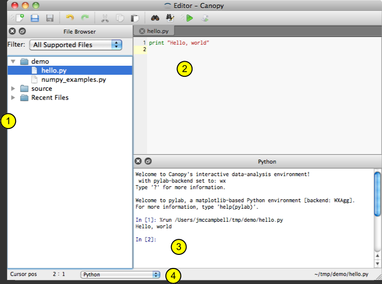
The screengrab below is borrowed from the Canopy documentation and should look something like your screen.

By default, the Editor will open a plain text file for editing (marked with a 2, above), with an area for output of code you run (3). It will also have a section for browsing and opening files on disk (1). None of these are really what we want. Close all of these by clicking the small (x) next to them.

Instead, we want to start a new IPython Notebook. Go to File>>New and choose "IPython Notebook." You should have a blinking cursor in a window that looks something like this.

In [ ]:

In IPython parlance, this is a cell. You can type Python code into a cell and then hit Shift+Enter to run the code in the selected cell. Things that you do in one cell persist, so that you can do some things in a cell to define a variable called my_stuff and then use my_stuff in a later cell. You can even save an IPython Notebook and it will preserve all the code you have written in various cells. Subsequent posts on using Python for HCUP data will depend heavily on IPython Notebooks, and will often include a notebook of the code in the post that you can open and use yourself.

For now, type the following and hit Shift+Enter to run the cell.

In [ ]:import pyhcup

If you are successful, the square brackets next to the "In" will have a number one in them, like this. If you get any other output, check for typos.

In [1]:import pyhcup

That's it for setup and configuration. We'll get more into actually using the PyHCUP library in the next post.

Sunday, December 1, 2013

HCUP and Python Pt 1: Background

This is the first post in a series on working with Healthcare Cost and Utilization Project (HCUP) datasets using Python and other open-source alternatives to SAS and SPSS, which are the two primary data tools supported by HCUP.

The United States Agency for Healthcare Research and Quality has a variety of large, de-identified hospital patient datasets available via its Healthcare Cost and Utilization Project (aka HCUP). They contain broad information on the diagnoses, duration, and type of treatment per patient for each visit, and slightly more detailed information on the type and volume of charges. Because of this, and because HCUP also makes available a unique identifier that can be used to “follow” a patient within a given state, many physicians, epidemiologists, economists, and other researchers use them as a source for retrospective analysis of outcomes and cost-effectiveness.

That said, the data sets can be large enough to cause some headaches. A single year’s worth of the “core” emergency department visit data for the state of California is about 10 million rows in 152 columns, and arrives from HCUP in a 5.8GB flat (non-delimited) file. What’s more, the number and width of columns supplied varies by the state supplying the data, and even varies by year within a given state.

To aid in parsing the datasets, HCUP provides loading program definitions in SAS and SPSS formats. Unfortunately, not everyone has SAS or SPSS available, and even some who do may have needs best met by other environments or prefer to use open source alternatives. Whatever your particular reasons, if you are interested in working with HCUP data without SAS or SPSS, you’ll need some other way to parse, manipulate, and integrate them.

In my case, I am using the Python programing language (especially the excellent pandas library) to parse HCUP data sets and do preliminary cleanup, then a PostgreSQL database for integration and long-term storage. Much of the Python code I am using is rolled into a package called PyHCUP, which is available on PyPI or simply through pip (pip install PyHCUP).

Over the coming weeks, I'll post more about how to use these and other tools to work with HCUP data.